Type inference under the hood
8 min read ·
If you’re into functional programming, you might have heard about Hindley-Milner. If not, it’s a type system that is the basis for most of the statically typed functional languages like Haskell, OCaml, SML, or F#. Here you can read some more about it, because in this article I won’t go into the details of H-M itself; I’ll focus on the type inference algorithm for H-M based type systems.
Nevertheless, it would be a pity if I blew my chance telling you my take on its most compelling aspects.
One of them is its completeness. Meaning it won’t go easy on you if you’d try to bypass it. You can’t tell it: shut up, I really want to do this typecast. It would yell, break your program at the compile-time, and make you want to stay away from it. But what doesn’t kill you makes you stronger. You can gain confidence — if your program finally compiles, it probably works. (It’s what I was saying to myself back when I was coding in Haskell). It not only allows you to catch errors earlier but often prevents them.
Another great feature is the ability to infer the type of expression without explicit declarations. That’s pretty much what’s this article is going to be about. I’ll do some overview of how type inference works for Hindley Milner type systems. Some of the examples are going to be in Haskell, but they are straightforward enough that no prior knowledge of Haskell is required. I aim to explain how the type inference algorithm for Hindley-Milner based type systems works under the hood without diving into in-depth details and formal definitions.
A word on functions
As I said, some examples in the article are in Haskell, so here comes a wrapping up about Haskell’s functions.
In Haskell, functions are first-class citizens, meaning that they don’t thumb their noses at the other data types. There’s nothing special about them. We treat them just as we treat other data types.
All functions in Haskell take one argument. More specifically — they take one argument at the time. Let’s take a look at the possibly most common example one could get:
add :: Integer -> Integer -> Integer
add x y = x + y
add :: Integer -> Integer -> Integer
add x y = x + y
How to read it in Haskellish?
Add is a function that takes an integer and returns the function that takes an integer and returns an integer.
Let’s put the brackets for more readability.
Add is a function that takes an integer and returns the (function that takes an integer and returns integer).
add :: Integer -> (Integer -> Integer)
add :: Integer -> (Integer -> Integer)
Like all the functions in Haskell, Add is curried.
Currying converts a function that takes n arguments into n functions that take one argument each.
Since all functions in Haskell take exactly one argument, you can think about
fun a b c = ... as the syntactic sugar for binding a lambda functions to fun: fun = \a -> \b -> \c -> ....
Type inference
Type inference means that types in a program can be deduced without explicit type annotations. The idea is that some information may not be specified, but the type inference algorithm can fill the gaps by determining the types from their usage.

Type inference was first invented by Haskell Curry and Robert Feys (for some lambda calculus stuff). Then J. Roger Hindley extended this algorithm, and couples years later, Robin Milner independently developed an equivalent algorithm — for the ML programming languages. Although practical type inference was developed for ML, it applies to other languages.
There is a broad spectrum to what degree a language can infer types, and in practice, almost no language supports full type inference. Core ML is very close, but it has some limitations when it comes to higher rank types.
Type inference supports polymorphism. The algorithm uses type variables as placeholders for types that are not known. Sometimes the type-inference algorithm may resolve all type variables and determine that they must be equal to specific types. Still, in other cases, the type of a function may not be constrained by the way the function is defined. In these cases, the function may be applied to any arguments whose types match the form given by a type expression containing type variable.
The idea behind type inference
Let’s say we have some simple function:
inc x = x + 1
inc x = x + 1
We know that the type of (+) is Int -> Int -> Int. Moreover, we also know that 1 has type Int. Having that knowledge, we can deduce that type of x must be Int. That implies that the type of inc is Int -> Int.
Now let’s take a look at another example and following reasoning:
f (g, h) = g(h(0))
f (g, h) = g(h(0))
- h is applied to 0 :: Int
- Based on ☝️ we can deduce type of h: h :: Int -> a, where a is some unknown type (type variable).
- g is a function that takes what h returns and return another thingy of the unknown type: g :: a -> b.
- Putting it altogether the first argument of f is going to be a -> b and the second Int -> a.
- Hence, function f takes the pair of (f, g) returns the same type the function g does which leads us to its final type:
f :: (a -> b, Int -> a) -> b
f :: (a -> b, Int -> a) -> b
Type inference vs type-checking
These terms are sometimes confused, so I’d like to clarify what’s the difference before we go further.
Standard type checking
js
js
What type checker does is examining the body of each function and then using declared types by the programmer is they match. Take a look at the above example. It would go through every usage of f and g functions and check two things:
- If the parameter is always of an integer type,
- If the functions return integers.
Type inference
js
js
What the type inference algorithm does is different. It goes through the program, examines the code without type information, and tries to infer the most general types that could have been declared.
Type inference algorithm
The algorithm consists of three steps:
- Assign a type or type variable to the expression and each subexpression. For known expressions, like +, - and so on, use the types known for these expressions. Otherwise, use type variables — placeholders for not known types.
- Generate a set of constraints on types, using the parse tree of the expression. These constraints are something like this:
if a function is applied to an integer, then the type of its argument is integer.
- Solve these constraints by unification — an algorithm for solving equations based on substitutions.
Now, let’s see this algorithm in action 🚀
Examples
#1
We’re going to start with a straightforward example, similar to what we had before. Below there’s a parse tree of the expression.
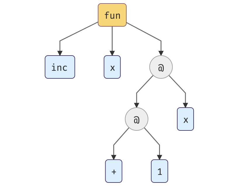
The root indicates that we have a function declaration here. The children are the expression bounded to the parent. In that case, we have add and x. The plus operator is treated as the prefix operator, not as the infix one. The nodes @ stand for function applications.
(+) 2 x is equivalent to x + 2. In Haskell, putting brackets around the operator converts it to the prefix function.
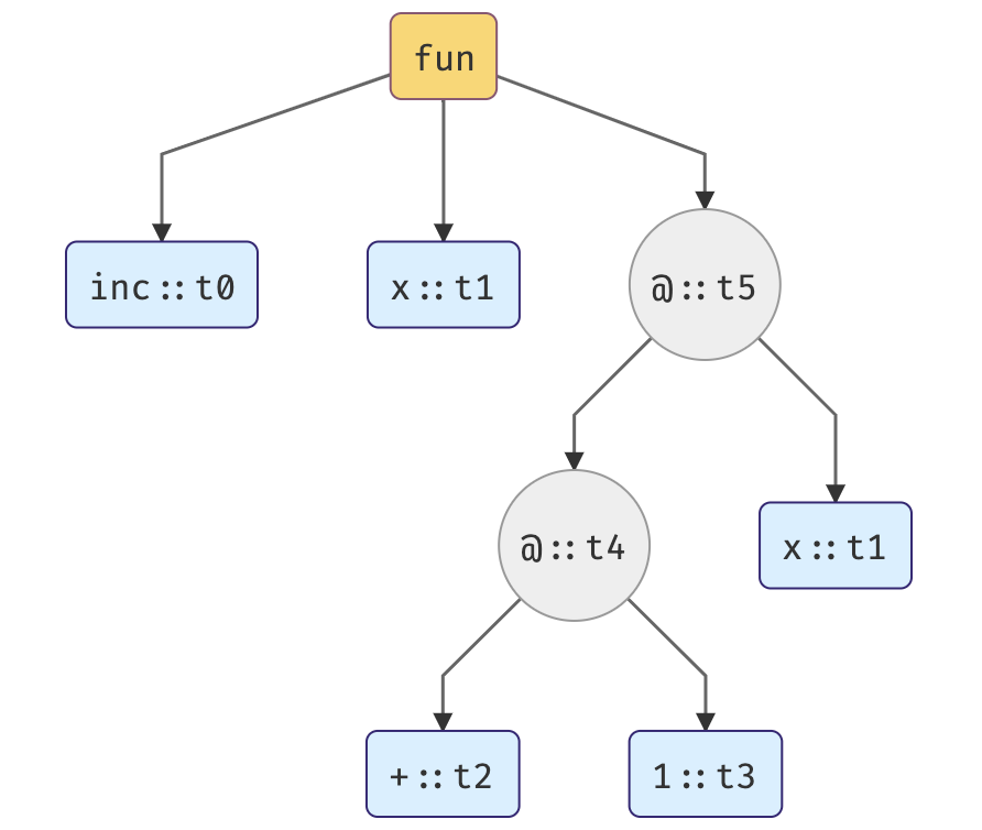
1. In the first step, we’re assigning type variables to each expression. Each occurrence of a bound variable must have the same type; in our case, variable x has the same type (t1) as a binding node.
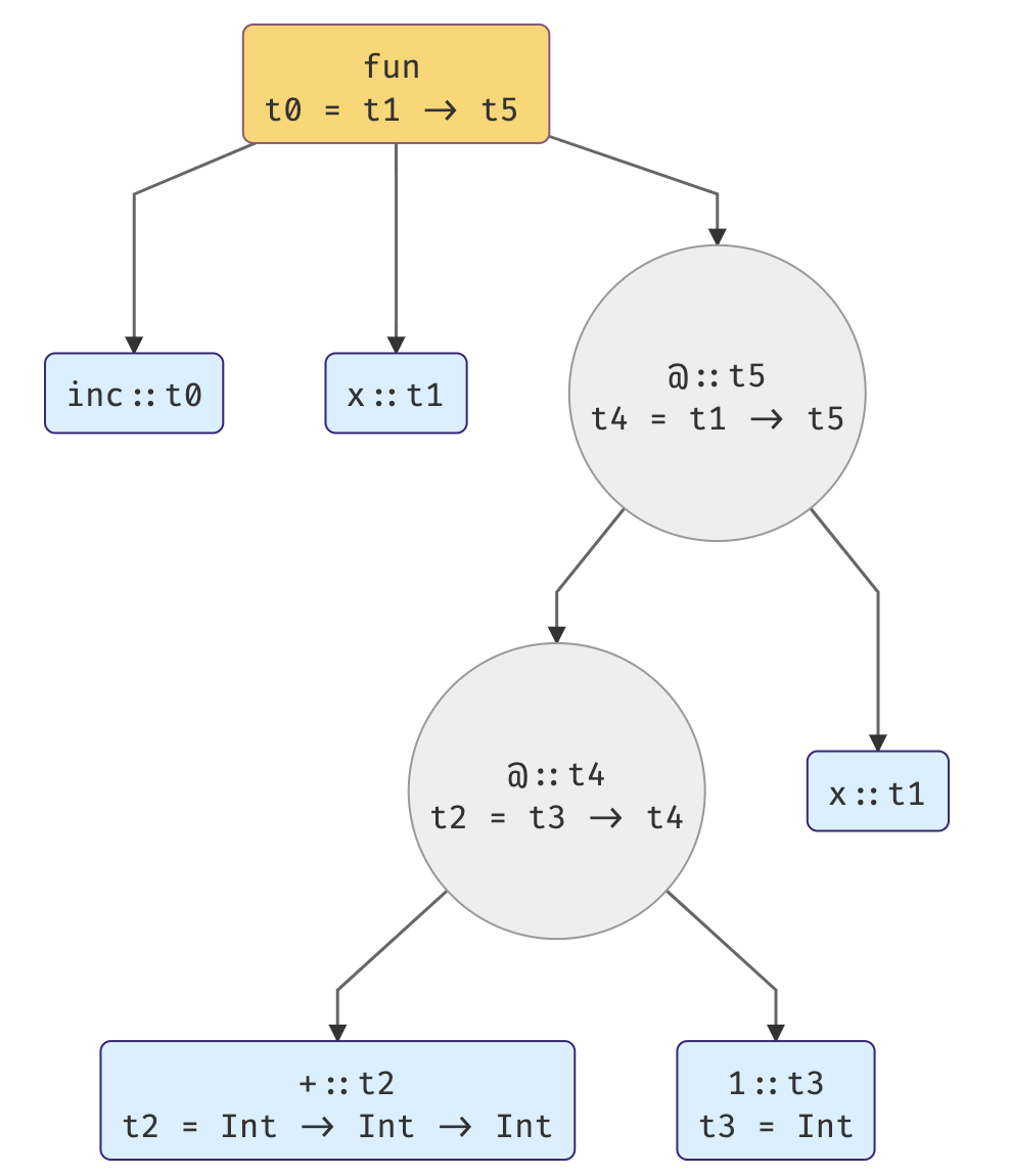
2. Now we’re generating a set of constraints on types.
Let’s gather all the constraints we can have at this point.
- t3 = Int because 2 is of type Int.
- t2 = Int -> Int -> Int, because the algorithm knows types of elementary functions like (+).
- Variable nodes don’t introduce any constraints, because the algorithm does not know anything but the values they represent, so for example: x stays as t1.
- @ nodes. If we have an expression like fun x, then we say that fun is applied to x and fun is of a function type. What’s more, the type of the whole expression fun x must be the same as the return type of fun. In our parse tree @ stands for fun a.
3. Final step — solving the constraints by unification.
The following list of constraints is just what we got from the second step.
1° t0 = t1 -> t6
2° t4 = t1 -> t6
3° t2 = t3 -> t4
4° t2 = Int -> (Int -> Int)
5° t3 = Int
Now, from the 4° and 5° we can imply the following equation:
6° t4 = Int -> Int (from 3° and 4°)
We still have t1 and t6 unsolved but thanks to the new equation 6° and 2° we can imply:
8° t1 = Int    (from 2° and 7°)
9° t6 = Int    (from 2° and 7°)
Hurrah! We have it all solved 🎉
t0 = Int -> Int
t1 = Int
t2 = Int -> Int -> Int
t3 = Int
t4 = Int -> Int
t6 = Int
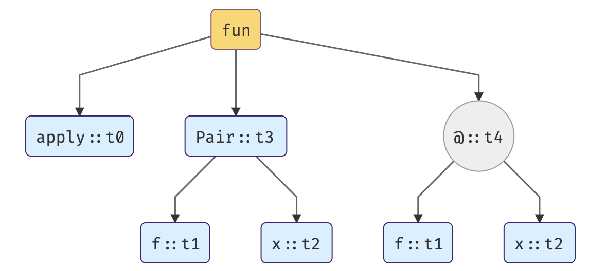
#2
Polymorphic functions this time. I won’t go into much details, hopefully you got the idea after the first example.
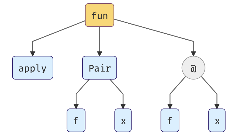
1. Assigning type variables to each expression.
2. Generating a set of constraints on types.
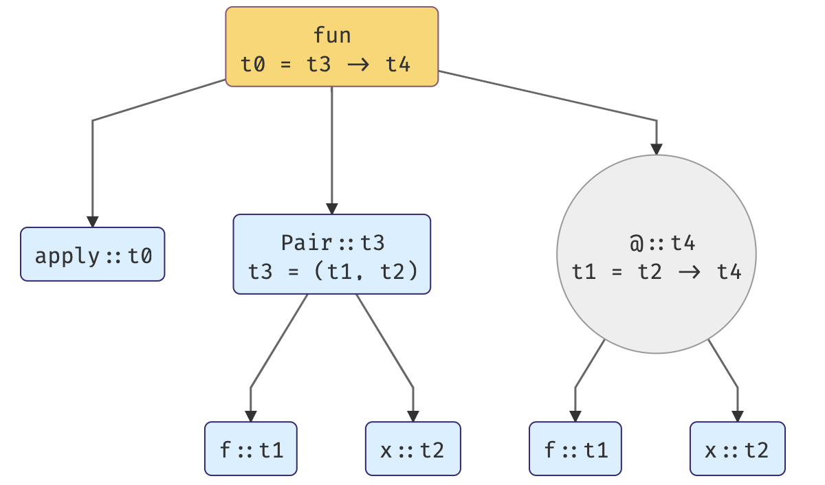
3. Solving the constraints by unification.
This is what we have on start:
1° t1 = t2 -> t6
2° t0 = t3 -> t6
3° t3 = (t1, t2)
Thanks to the equation 3°, we can substitute t3 in equation 1°:
4° t0 = (t1, t2) -> t6
And then use 1° to substitute t1 in 4°:
5° t0 = (t2 -> t6, t2) -> t6
And the above stands for the type of our polymorphic function! 🎉
Complexity
The time complexity for this algorithm was proven to be exponential. However, it’s mostly linear in practice, but exponential in the depth of polymorphic declarations.
Summary
As I wrote at the beginning, it was supposed to be a super brief inference algorithm explanation. I hope somebody can benefit from this.
Thank you for your attention! Feel free to correct me if I got something wrong 😅